Making Interactive Maps with whampy

You can make interactive maps of the WHAM data where you can click on the map and have a spectrum plotted from the nearest WHAM pointing using the click_map method:

>>> import matplotlib.pyplot as plt
>>> %matplotlib notebook
>>> from whampy.skySurvey import SkySurvey
>>> survey = SkySurvey()

>>> click_map = survey.click_map()

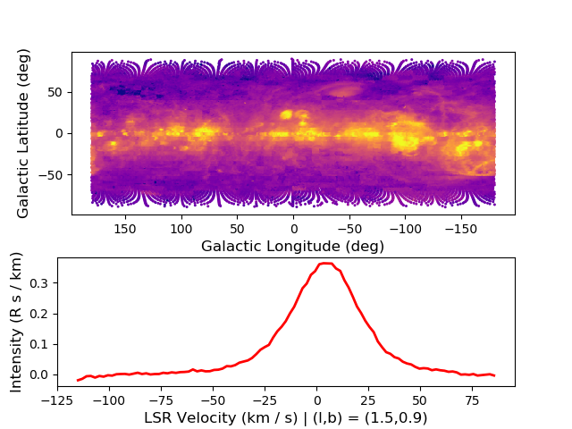
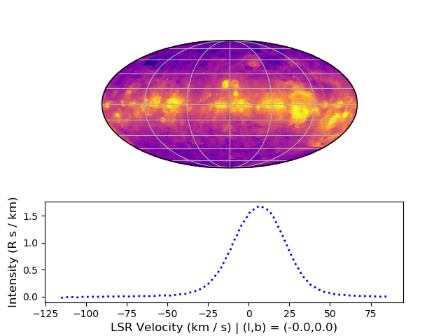
click_map will accept and pass keywords to intensity_map. You can also pass in your own set of figure and axes instances to customize the orientation, shape, and size of axes. The example below uses the optional dependency cartopy and this package will need to be installed separately following the instructions on its documentation:

>>> import cartopy.crs as ccrs
>>> fig = plt.figure()
>>> image_ax = fig.add_subplot(111, projection = ccrs.Mollweide())

>>> click_map = survey.click_map(fig = fig, image_ax = image_ax,
...             spectra_kwargs = {"c":'b', "ls": ":"})

Making Interactive Maps that overplot Additional Spectra

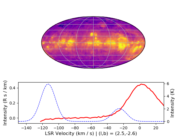
You can also make these interactive maps and have clicks additionally plot another spectra from a different source. This additional data can be from a FITS Data cube or another SkySurvey object for other wavelength WHAM observations.

This feature uses the optional dependency spectral-cube package to handle FITS data cubes and this package will need to be installed separately following the instructions on its documentation. spectral-cube can read in 3D datacubes that are regularly gridded with an NAXIS = 3 keyword set in its header and that contains a spectral axis (velocity, wavelength, frequency).:

>>> fits_cube_path = "hi_data_cube.fits"
>>> fig = plt.figure()
>>> click_map = survey.click_map(fig = fig, over_data = fits_cube_path)

You can set the velocity range to be static to focus on certain regions if desired:

>>> spec_ax = click_map.line_ax
>>> spec_ax.set_xlim([-150,30])